4 Value Added Models

Value-Added Models (VAMs) are statistical tools designed to measure the impact of educators, schools, or programs on student learning outcomes. The central idea is straightforward: how much growth did a student show over time, and how much of that growth can reasonably be attributed to their teacher or school, rather than other factors?

If a student scored 60 on a math test last year and 75 this year, a simple comparison might suggest a 15-point improvement. VAMs go a step further by asking, “How does this improvement compare to what we would have expected, based on the student’s prior performance and background?”

To do this, VAMs use complex statistical models that factor in things like prior achievement (often from multiple years of test data), student demographics (e.g., socioeconomic status, language proficiency), and school characteristics (like average class size or funding levels). VAMs are typically used in large-scale educational assessments and accountability systems. They inform professional development, curriculum design, and even in some cases, parent decisions.

It’s important to note that VAMs don’t measure everything. They focus on academic growth, usually based on standardized test scores, and they rely on assumptions made by analysts about what factors matter most.

The Simple Covariate Model

Let’s begin with the most basic type of value-added model: the Simple Covariate Model. It compares students’ current achievement with their past performance, while also adjusting for a few background characteristics. It’s a regression-based model, which means it looks for relationships between variables. Specifically, how prior test scores and other factors predict current achievement.

How Does It Work?

The model takes data on students' previous test scores and relevant demographic variables (like socioeconomic status or English learner status) as input. It uses those inputs to predict what a student should score this year, based on what similar students have scored historically. It then looks at the difference between the student’s actual score and their predicted score. That difference is considered the “value added” by the teacher or school.

Imagine a student predicted to score 70 but ends up scoring 75. That 5-point gain is potentially attributable to something in the teaching environment, this may be instructional quality, or maybe curriculum design.

Why Use It?

It’s simple, transparent, and relatively easy to implement. Educators can understand it without needing a PhD in statistics. This model introduces the concept that we shouldn’t evaluate educators based on raw achievement alone.

What Are the Limitations?

Because it compares performance across classrooms or schools, there’s always a risk that the results reflect differences in students more than differences in teaching.

Still, this model is a useful starting point. It encourages educators and policymakers to think beyond surface-level scores and focus on growth, something that’s far more relevant for helping students improve.

The Fixed Effects Model

Now that we’ve covered the basics with the Simple Covariate Model, let’s move a step further with the Fixed Effects Model. This model is designed to answer an even more pointed question: How much of a student’s academic growth can we attribute specifically to their teacher, when we control for everything else we can’t easily measure?

What’s Different Here?

The Fixed Effects Model also looks at test score growth over time, but instead of just adjusting for prior scores and demographics, it controls for all student-level characteristics that don’t change over time. Think personality, family environment, motivation, and even innate learning ability. These factors don’t usually vary much year to year, and the fixed effects approach assumes that if we observe a student across multiple years and multiple teachers, we can essentially "subtract out" those consistent traits. The model works best when students change teachers over time, which allows it to compare how the same student performs with different teachers.

Let’s say we have a student named Maya.

• In Year 1, she’s in Mr. Smith’s class and scores 80 on the state math test.
• In Year 2, she moves to Ms. Johnson’s class and scores 90.

A Simple Covariate Model would be interpreted as: “Great, she improved! Let’s adjust for background factors and give some credit to Ms. Johnson.” But the Fixed Effects Model would go further: “Wait, how did other students do under Mr. Smith and Ms. Johnson? And how has Maya performed across multiple years and subjects? Let’s use all that to better estimate how much Ms. Johnson’s teaching contributed to that jump.” Over time, if Maya consistently shows stronger gains with certain teachers, the model picks up on that while keeping her underlying traits constant.

Why Use This Model?

Because it’s better at isolating true teaching effects. It controls for all the static factors that might otherwise bias our conclusions. This is especially useful in research and in large districts where students have long achievement records and rotate among teachers.

It’s also more robust when used in evaluations. Principals, districts, or researchers can be more confident that they’re not just rewarding teachers who happen to work with higher-performing students year after year.

What’s the Tradeoff?

You need a lot of longitudinal data, several years of student test scores across multiple teachers. Small schools or districts might struggle with that. The math also gets more complex. It’s less intuitive to interpret without some statistical background

The Random Effects (Hierarchical Linear) Model

After the Fixed Effects Model, you might be wondering: what if we don’t want to control for every individual trait, but instead want to understand patterns at different levels (student, classroom, school, even district)? That’s where the Random Effects Model ( also called Hierarchical Linear Model ) comes in. It helps us understand how performance varies across nested layers of the education system, like Russian dolls, each layer sitting within the next.

How Does It Work?

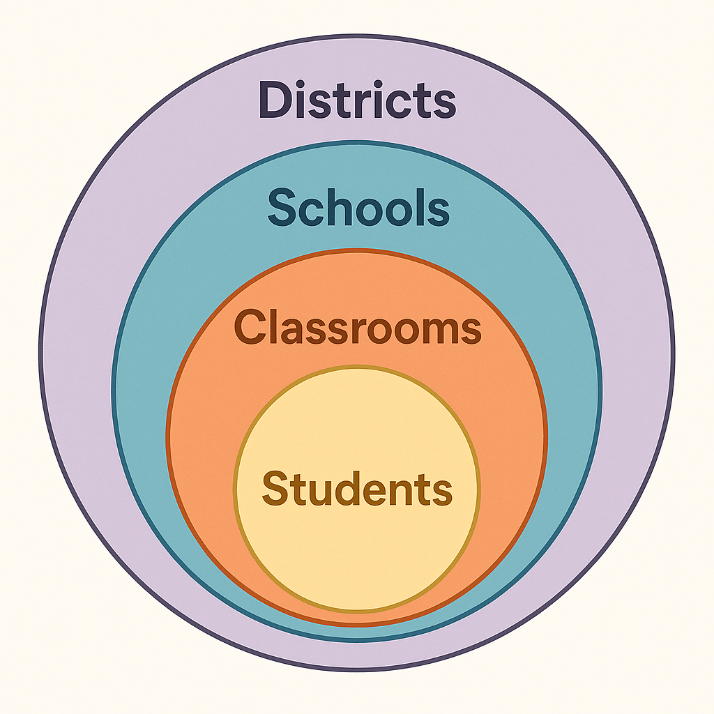
Imagine students nested within classrooms, classrooms within schools, and schools within districts. HLM treats these as hierarchical levels, each contributing to the overall variation in student achievement. It breaks down the question: Where is the growth coming from?

• How much variation is due to the individual student?
• How much is due to the teacher or the classroom?
• How much can be traced to the school or district?

It assumes that differences in teaching effectiveness, for instance, come from a broader distribution of teacher performance, and it estimates each teacher’s contribution based on that distribution.

Let’s return to Maya, our student from earlier.

• Maya’s in a 5th-grade math class in School A.
• Her classmates also took the test, and the average gain in the class was +10 points.
• Meanwhile, across the district, 5th-grade students in other schools saw an average gain of +5 points.

The Random Effects Model would evaluate not just Maya’s gain, but how her classroom's gain compares to the school and district averages. It would estimate how much of that difference is likely due to her teacher’s impact, relative to what’s normal across all teachers and schools. This model would also consider how much variation exists across schools or even districts. It’s particularly useful when trying to identify systemic patterns, not just individual teacher performance.

Why Use It?

It balances fairness and precision: The model reduces the risk of over-attributing high or low results to one teacher based on limited data.

It works well with uneven data: In real-world settings, some teachers have more students than others, or students with different backgrounds. HLM handles that imbalance better than other models.

What’s the Tradeoff?

Complexity: This model is statistically advanced and can be hard to explain to non-research audiences.

Assumptions Matter: It assumes that teacher and school effects come from a shared distribution. If that’s not true in your system, estimates can be misleading.

Data Quality: Like the Fixed Effects Model, it still depends on strong longitudinal data and consistent testing practices.

Student Growth Percentiles (SGPs)

So far, we've talked about value-added models that use predictive frameworks to estimate how much progress a student should have made. But what if we drop the prediction altogether and focus on relative growth: comparing students to their academic peers?

The Student Growth Percentile (SGP) model is a more descriptive, non-parametric tool that answers a straightforward question: Compared to academically similar students, how much progress did this student make?

How does it work?

The SGP method groups students based on their prior test scores, so a student like Maya is compared only to other students who scored similarly in the past. This group is called her academic peer group. SGP assigns a percentile rank (0–100) to each student’s growth. If Maya’s SGP is 75, it means she grew more than 75% of the students who had the same starting point. The model doesn’t make assumptions about background characteristics, schools, or teachers. It just focuses on test score improvement relative to similar students.

Say two students, Maya and Leo, both scored 60 in math last year.

• This year, Maya scored 75, while most of her peers scored between 68 and 72.
• Maya’s growth is high compared to her peer group—her SGP might be 85.
• Leo scores 65, which places him behind most of his peers—his SGP might be 25.

This tells us something very specific: how much progress each student made relative to others who previously had the same performance. It’s a simple way to track growth without the complexity of regression-based models.

Why Use SGP?

Simplicity and transparency: Educators and parents can easily interpret percentiles. If a student is in the 80th growth percentile, that’s an intuitive signal that they’re making strong progress.

Fair comparisons: It compares students to others with similar prior scores.

What’s the Tradeoff?

No causal inference: SGPs describe growth, but they don’t explain why it happened. You can’t say whether the teacher, the curriculum, or something else caused the growth.

Less control for context: Unlike value-added models that adjust for demographics or school-level effects, SGPs don’t account for many external variables.

Potential misuse: On their own, SGPs aren’t designed for high-stakes decisions about educators, but they sometimes get used that way, which can be problematic.

Wrapping It all up...

Each value-added model we’ve discussed offers a different lens:

• Simple Covariate Model: Easy to understand, but limited in what it controls for.
• Fixed Effects Model: Focuses on isolating teacher impact by controlling for unchanging student traits.
• Random Effects (HLM): Captures influence across nested levels—classrooms, schools, districts.
• SGPs: Offers clear, comparative insights into growth without heavy statistical assumptions.

References

Amrein-Beardsley, A. (2008). Methodological concerns about the Education Value-Added Assessment System. Educational Researcher, 37, 65–75.

Amrein-Beardsley, A., Pivovarova, M., & Geiger, T. (2016). Value-added models. Phi Delta Kappan, 98, 35–40.

Bi, Y.-F. (2012). The research and application of value-added models for teachers.

Gray, L. (2019). Value-Added Models and other forms of teacher abuse. In Educational Trauma (pp. 1–10)

Koedel, C., Mihaly, K., & Rockoff, J. E. (2015). Value-added modeling: A review. Economics of Education Review, 47, 180–195.

Martineau, J. A. (2006). Book review: Value Added Models in Education: Theory and Practice. Applied Psychological Measurement, 30, 249–252

McCaffrey, D. (2010). Value-Added Models. In International Encyclopedia of Education (pp. 489–494)

Nakamura, Y. (2013). A primer on value-added models: Towards a better understanding of the quantitative analysis of student achievement.